
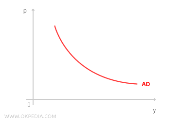
Building the aggregate demand curve
The aggregate demand curve is constructed using the IS-LM model by linking each macroeconomic equilibrium (e) to its corresponding price level (p). In the IS-LM framework, the main variables are income (y) and the interest rate (i), while the price level (p) is treated as an external factor. The process of building the aggregate demand curve from the IS-LM model can be visualized on a Cartesian plane by examining how price level changes affect the system.
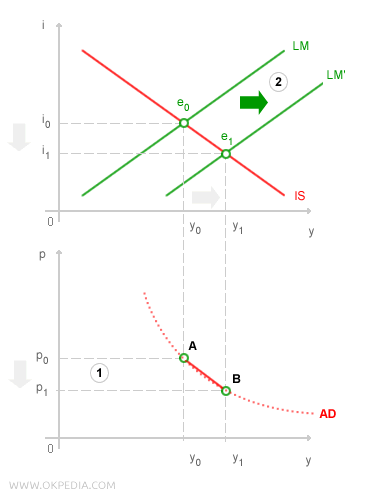
The initial equilibrium, e0, corresponds to an income level of y0 and a price level of p0. On the income-price diagram (the lower graph), the coordinates (y0, p0) mark point A. A reduction in the price level from p0 to p1 (phase 1) increases the real money supply (M/P) in the economy. On the income-interest rate diagram (the upper graph), this monetary expansion (ΔM/P) shifts the LM curve to the right (phase 2). As a result, the interest rate drops from i0 to i1. The lower interest rate stimulates domestic demand by encouraging investment, which drives income higher from y0 to y1. The adjustment process concludes when the economy reaches a new macroeconomic equilibrium (e1) at a lower interest rate (i1) and a higher income level (y1). Once the new equilibrium income (y1) is identified, it is projected onto the income-price diagram (the lower graph) to locate point B at (y1, p1). By connecting points A and B, the aggregate demand curve (AD) can be plotted. By varying the price level, it is possible to trace the entire aggregate demand curve (AD) starting from the macroeconomic equilibrium described by the IS-LM model. Each point on the AD curve represents equilibrium in both the goods and money markets.
Algebraically, the relationship between income (y) and price level (p) under macroeconomic equilibrium is derived by combining the IS and LM equations from the IS-LM model. The equation for the AD curve is as follows:
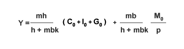
In this equation, C0, I0, and G0 represent autonomous consumption, autonomous investment, and government spending, respectively. Together, these form autonomous demand. The parameter m represents the income multiplier (1 / 1-c). The variable M0 refers to the nominal money supply, while P denotes the price level. The ratio M0/P indicates the real money supply.

The construction of the aggregate demand (AD) curve based on the IS-LM model creates a connection to the AD-AS model, introducing the price level (P) into the analysis of macroeconomic equilibrium. This connection allows economists to examine the impact of policy changes without relying on the assumption of constant prices.


