Investment Function

The investment function represents the economic relationship between the volume of investments and the market interest rate. It's an integral part of the IS-LM model. There exists an inverse relationship between investments and interest rates. An increase in the interest rate raises the cost of money. Under similar conditions, for securing a loan, investors need to pay more interest to the lender. This leads to a decrease in the amount of investments made by a company (investment expenditure). Conversely, a decrease in interest rates has the opposite effect, lowering the cost of money and enabling companies to obtain financing with less interest burden. This encourages entrepreneurs to increase investment spending. In the IS-LM model, the investment function can be written as follows:

I = I₀ - b·i

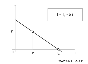
Investment spending (I) is determined in the following manner. Starting from the investment value I0, which would exist if the interest rate were zero (i = 0), we subtract the current interest rate (i) multiplied by the sensitivity (b) of economic operators to interest rate changes (b > 0). For instance, with no sensitivity to interest rate changes (b = 0), investment spending is independent of interest rate fluctuations. However, when the variable (b) is significantly high, investment spending becomes highly dependent on interest rate changes. The investment function can be graphically represented on a Cartesian diagram, plotting investment values on the x-axis and interest rate on the y-axis.

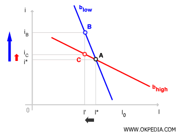
In a Cartesian plane, the investment function shows a decreasing trend. An increase in the interest rate (i) reduces investment spending (I) of companies, and vice versa. The intercept point I0 on the x-axis indicates the investment value if the interest rate were zero (i = 0). For example, an interest rate i* leads to an investment spending I*. The graphical representation also allows for a better analysis of sensitivity (b) to interest rate changes. The following diagram illustrates two contrasting cases:

In the investment function with high sensitivity (b_high), a slight change in the interest rate causes a significant variation in investment spending (I). The investment function appears almost flat. In contrast, in the investment function with low sensitivity (b_low), a change in the interest rate leads to a minimal variation in investment spending. The demand for investments is more rigid. For instance, to reduce investments from I* to I', in the highly sensitive investment function (b_high), only a small change in the interest rate from i* to i_C is required. The equilibrium shifts from point A to C. In the less sensitive investment function (b_low), however, a significant change in the interest rate from i* to i_B is needed as the investment decisions of companies are less influenced by the interest rate level. The equilibrium point moves from A to B.

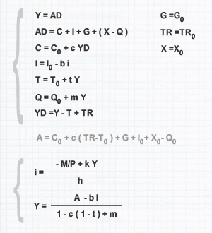
From the Income-Expenditure Model to the IS-LM Model. In the income-expenditure model, the level of investments is considered constant (an exogenous variable) and determined by companies' long-term expectations. Incorporating the investment function into the income-expenditure model links the interest rate with variations in aggregate demand (AD) and income (Y) through induced changes in investment spending (I).

Since the interest rate (i) is also a determining factor in the money market, this allows for the identification of an interest rate level (i*) that simultaneously equilibrates both the real investment/savings market (IS schedule) and the money market (LM schedule). The introduction of the investment function enables the transition from the income-expenditure model to the IS-LM model.