IS Curve

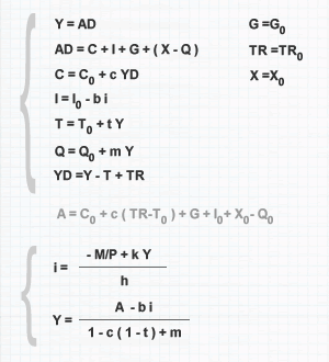
The IS curve represents the equilibrium combinations of income (Y) and interest rate (i) in the IS-LM model. The IS curve (IS schedule) is the set of equilibrium points in the goods market. At every point on the IS curve, aggregate demand (AD) equals income (Y). To construct the IS curve, one must start from the IS-LM model. In the IS-LM model, the income equation is as follows:

Y = C + I + G + TR - T + X - M

The income equation (Y) in the IS-LM model is identical to that of the income-expenditure model. Income is determined by consumption expenditure (C), investment expenditure (I), government spending (G), exports (X), and, inversely, by taxation (T). What differs between the goods market in the IS-LM model and the income-expenditure model is the investment function. In the income-expenditure model, current investments (I) are an exogenous variable and are determined by firms' long-term expectations. In the IS-LM model, however, current investments (I) are inversely related to the interest rate. The investment function in the IS-LM model is as follows:

I = I₀ - bi

Given that government spending (G), transfers (TR), imports (M), and exports (X) are exogenous variables (constants) and that the other variables of the economic model are as follows:

C = C₀ + cYd
T = T₀ + tY
Yd = Y - T + TR

We can rewrite the income equation by substituting the consumption (C), investment (I), and taxation (T) variables with their respective determining equations. By highlighting the income variable (Y) and after some simple algebraic steps that we omit, we obtain an equation that relates the level of income (Y) to the interest rate (i).

The IS equation can be represented on a Cartesian diagram by placing income on the x-axis and the interest rate on the y-axis. Points on the IS curve are equilibrium points. They are combinations (Y, i) that bring the goods market into equilibrium.

In the previous diagram, three distinct situations are represented. At a given interest rate (i), the income level Y' is lower than aggregate demand (AD). From this, we deduce that all points to the left of the IS curve are non-equilibrium situations of excess demand relative to income. The income level Y" is, instead, higher than aggregate demand. Thus, all points to the right of the IS curve are non-equilibrium situations of excess production (excess supply). Finally, the income level Y is the only equilibrium point which, starting from the interest rate i, equates aggregate demand to income.

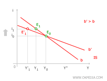
Slope of the IS Curve. The IS curve has a negative slope due to the inverse relationship between investment expenditure (I) and the interest rate. As the interest rate (i) increases, firms face higher interest costs for financing, leading them to reduce their investment activities. Conversely, when the interest rate decreases, the cost of financing lowers, encouraging firms to ramp up their investments (I). Investment expenditure (I) is a component of aggregate demand, and thus, any change in investment expenditure causes (under ceteris paribus conditions) a change in the same direction in aggregate demand (AD) and, ultimately, in the level of income (Y). The flatter the IS curve, the more sensitive (b) the investment expenditure is to changes in the interest rate, and vice versa.

Fiscal Policy. Public spending (G) and taxation (T) are variables in the numerator of the income multiplier. Hence, any variation in these variables shifts the IS curve rightward or leftward. For example, an increase in public spending boosts aggregate demand, ceteris paribus, leading to an expansive effect on national income. This results in a rightward shift of the IS curve.