Stability of macroeconomic equilibrium
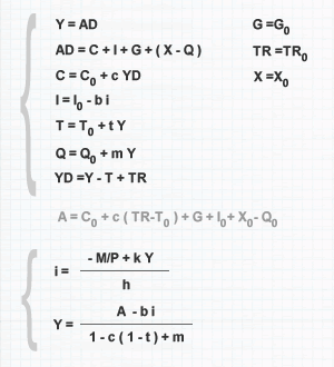
The stability of macroeconomic equilibrium refers to an economic equilibrium where key variables remain unchanged over time. An economic equilibrium is considered stable when, ceteris paribus, once the equilibrium conditions are met, no further changes occur. For example, the IS-LM model is in equilibrium where the IS curve intersects the LM curve, indicating that both the goods market and the money market are balanced. In cases of instability, the equilibrium conditions tend to shift progressively.

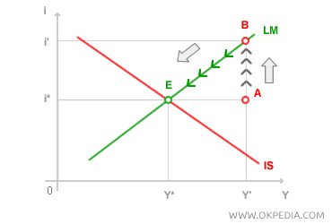
As an example, situation A represents disequilibrium. Point A lies outside both the IS and LM curves, indicating an imbalance in both the goods market and the money market. Specifically, point A shows an excess demand for money (L>M) and an oversupply of goods (Y>AD). The excess demand for money leads agents to sell off their assets in order to increase their cash reserves. This causes asset prices to drop and drives up the interest rate. As this adjustment process unfolds, the equilibrium shifts to point B, which lies on the LM curve, meaning the money market is now balanced. However, point B is still not a stable equilibrium. While the money market is balanced, the goods market continues to experience excess production relative to demand. As a result, production (Y) is reduced, and the equilibrium point moves leftward. To prevent an excess supply of money, the interest rate tends to fall as production declines, eventually aligning with the IS curve. The adjustment process concludes at point E, where both the goods market and the money market are in equilibrium. Point E represents a stable equilibrium, as no further market forces act to alter it.
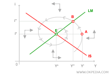
 Dynamic adjustment process. The dynamic adjustment process towards a stable equilibrium is more complex than what has been described so far. In the previous example, we assumed the money market adjusts rapidly, followed by the goods market only after the temporary equilibrium at point B is reached. In reality, both adjustment processes, while occurring at different speeds, happen simultaneously over time. The dynamic adjustment process towards equilibrium is illustrated as follows:

The dynamic adjustment process towards equilibrium traces a spiral on a Cartesian plane. As you can see, during the transition from situation A to situation B, the interest rate rises (+Δi) while production falls (-ΔY). This adjustment process continues, driven by the forces of the money and goods markets, drawing a spiral path that gradually converges towards the macroeconomic equilibrium at point E.

