Supply curve

The supply curve is a graphical representation of the economic supply of a good or service on a Cartesian plane. It is based on a mathematical function where price is the independent variable (input) and the quantity produced is the dependent variable (output).

q=f(p)

The price and quantity produced of a good help calculate the firm's revenue. Combined with economic costs, this allows for the determination of profit. Naturally, a firm's objective is to maximize profit. Therefore, other factors remaining constant, the higher the market price of a good, the greater the quantity a firm is willing to produce. This is why the supply curve typically slopes upward. For instance, if the price is €1.00, the firm produces 100 units per day. If the price increases to €2.00, the firm boosts production to 140 units per day, and so forth.

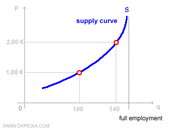
The supply curve has a positive slope due to the law of supply. According to this principle, an increase in price results in a higher quantity of goods or services supplied, and vice versa.

When constructing the supply curve on a Cartesian plane, all other environmental variables, such as technology, input prices, and the prices of other goods, are assumed to be constant.

Position of the Supply Curve

The position of the supply curve is influenced by production costs and technology. On the graph, the supply curve can shift rightward or leftward depending on changes in production conditions (see shift of the supply curve). There are two possible scenarios:

1. Contraction of supply. An increase in production costs shifts the supply curve to the left. For example, a rise in labor costs, production taxes, and so on.
   
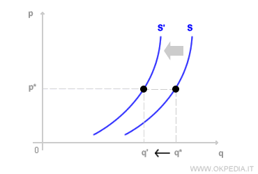
2. Expansion of supply. A reduction in production costs shifts the supply curve to the right. This rightward shift allows the firm to produce a larger quantity of the good (q).

   

What causes the supply curve to shift? The supply curve shifts to the right when technological advancements (technological progress) reduce production costs, taxes decrease, or the cost of labor, production factors, or capital declines.

Convex Shape of the Supply Curve

The shape of the supply curve depends on the market environment in which the firm operates, the production function, and the production costs. The supply curve often has a convex shape due to the behavior of returns to scale and the long-term average cost curve.

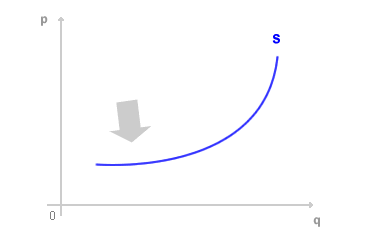
• Initial segment of the supply curve. In the initial part of the curve (horizontal segment), the plant capacity is underutilized, and returns to scale are increasing. Under these conditions, the firm is incentivized to increase production more than proportionally to changes in price. This makes the supply curve very elastic to price variations in this segment.
  
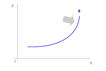
• Final segment of the supply curve. In the final part of the curve (vertical segment), the plants are operating near full capacity (full employment), and returns to scale are decreasing. Here, the firm increases production less than proportionally to price changes, making the supply curve progressively less elastic and more rigid to price variations. It culminates in a vertical line when the maximum capacity is reached.
  

Market Equilibrium. The supply curve on its own is not sufficient to determine price or equilibrium. To find market price and equilibrium, the demand curve must also be considered. The intersection of the supply and demand curves represents a state of equilibrium where the quantity produced matches the quantity consumers are willing to buy.

Constructing the Supply Curve

In the short run, the supply curve of a competitive firm corresponds to the portion of the marginal cost curve that lies above the average variable costs.

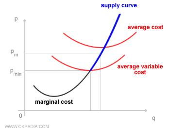
When the selling price falls below average variable costs, no supply is produced as it would result in a loss.

In the short term, fixed costs remain unchanged. Therefore, the firm focuses on average variable costs (rather than average costs) as the reference.

In perfect competition, firms are price-takers. In a perfectly competitive market, individual firms cannot set the selling price because it is determined by the market, and no single firm can influence it. The firm can only decide on the quantity of production. According to the profit maximization rule (MC = MR), the optimal choice for a firm in perfect competition lies along the marginal cost curve where it intersects the market price. An example of perfect competition can be seen in the global agricultural market.

The long-run supply curve is determined by the intersection of the marginal cost curve with the average cost curve.

In the long run, the firm also takes into account the fixed costs of its facilities.