Aggregate Supply Curve

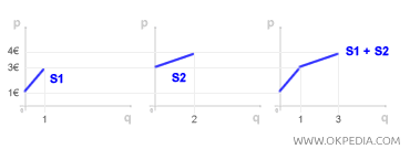
The aggregate supply curve illustrates the relationship between the total quantity of goods produced and supplied by firms in a specific economic sector and the market price level. For any given price level, this curve aggregates the quantities supplied by individual firms (aggregate quantity). By adjusting the price, the total quantity of goods offered in the market can be determined, allowing for the construction of the short-term aggregate supply curve. The example below demonstrates the aggregate supply curve in a market comprising just two firms.

The construction of the aggregate supply curve is a cornerstone of macroeconomics, which focuses on the analysis of aggregate economic indicators. Aggregate supply refers to the total output (or production) that firms are willing to produce and supply at various price levels. Typically, the aggregate supply curve slopes upward, reflecting a positive relationship with price. The shape of the curve depends on market conditions and remains a topic of debate among different economic schools of thought. In macroeconomic models (e.g., the AD-AS model), the aggregate supply curve is depicted on a Cartesian plane, showing the interplay between price (p) and income-output (y). It is commonly referred to as the AS curve (or AS schedule).

The AS curve determines equilibrium output (y) based on price levels and is derived from the combined production functions of all firms operating in the economic system. Its shape is influenced by factors such as technology and the cost of production inputs.

Constructing the Aggregate Supply Curve. The aggregate supply curve (AS curve) is built on the principles of profit maximization and the marginal productivity of production inputs. Each firm determines its output level to maximize profit. All else being equal, an increase in price raises total revenue from production inputs, encouraging firms to increase output. As a result, the supply (or production) function is positively correlated with price.