Cost Function

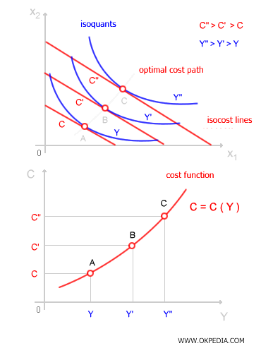
The cost function describes the relationship between output and the minimum cost required to produce it. Given a production function with two input factors, y = f(x₁, x₂), the cost function determines the lowest possible production cost C* for any given level of output Y.

C = C(Y)

Graphically, the minimum cost is represented by the point where an isocost line is tangent to an isoquant curve (optimal allocation of inputs). As we know, isoquant curves illustrate different combinations of input factors (x₁, x₂) that yield the same level of output Y. By analyzing a set of isoquants, we can visualize the corresponding output levels Y of a production function. By connecting the points where isoquants touch isocost lines, we derive the (C, Y) values needed to plot the cost function.

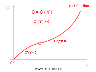
The cost function shows how total cost C changes as output Y varies. Mathematically, the cost function is always increasing with respect to production level, meaning its first derivative is positive.

C'(x) > 0

In simpler terms, producing more output always requires using more input factors, which drives up total production costs. However, the rate at which costs increase isn't always straightforward and depends on the second derivative of the cost function C"(x), as well as marginal and average costs. Typically, when output Y rises, the increase in production costs is initially gradual (C"(x) < 0) but becomes steeper at higher levels of production (C"(x) > 0). In other words, costs grow at a slower rate at lower production levels but escalate more rapidly beyond a certain threshold.

When constructing the isocost function, we assume that input prices remain constant regardless of the level of production. In this case, total spending is tied to the volume of output Y rather than the quantity of inputs purchased. This assumption holds when a firm's production level is too small to influence input prices. On a graph, this is represented by the fact that isocost lines maintain the same slope at all levels of output Y.