Developing the Aggregate Supply Curve

The development of the aggregate supply curve is rooted in the production decisions of individual firms operating within a market or economic system. In a competitive market economy, each firm determines its production level (y) with the goal of maximizing profits. For simplicity, let’s focus on the production function of a single firm that produces one product (y) using only one input: labor.

y = f(L)

In microeconomics (theory of the firm), the profit equation for a firm is expressed as:

π = p y - w L

The profit (π) of a firm is the difference between its total revenue—calculated as price (p) multiplied by output (y)—and its total cost, represented by wages (w) multiplied by the amount of labor input (L). A firm will continue increasing production as long as each additional unit of output raises profit (Δπ > 0). Mathematically, the production level that maximizes profit is determined by setting the first derivative of the profit function (π') with respect to labor equal to zero.

π' = 0

The algebraic expression for profit maximization can also be rewritten as:

π' = p f'(L) - w

In other words, profit is maximized when the marginal revenue, p f'(L), generated by selling one additional unit equals the firm’s marginal cost, which in this case is the wage (w).

p f'(L) = w

This equation also highlights the equality between marginal productivity (f'(L)) and the real wage (w/p).

f'(L) = w/p

This relationship explains how a firm adjusts its behavior in response to price changes. Assuming wages (w) are an exogenous variable, an increase in the product’s price (p) lowers the real wage and, indirectly, encourages greater use of the production input (L). This, in turn, leads to increased output (y).

Δy = f(ΔL)

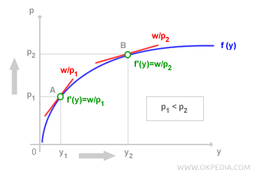
The graph below illustrates how a price increase from p₁ to p₂ affects a firm’s output (y). Starting from an initial point (A), the drop in the real wage from w/p₁ to w/p₂ enables the firm to raise its output (y), reaching a lower marginal productivity level, f'(y), at point B.

Assuming the principle of diminishing marginal productivity in both the production function and labor, variations in price (p) allow the firm to determine its optimal output level (y). By plotting pairs of (y, p) values on a Cartesian plane, the points can be connected to form the firm’s supply curve.

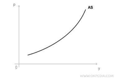
The supply curve of a product slopes upward with price. The process of selecting production levels follows the same profit-maximization logic for all firms. To build the aggregate supply curve, this principle is applied to sum the output of all firms (y₁ + y₂ + ... + y_n) at each price level (p). By plotting the total output of all individual firms on a Cartesian plane, the aggregate supply curve (AS curve) is derived. As prices rise, real wages (w/p) decrease, driving higher employment (L) and boosting total output (y) in the economy. Like the individual supply curves, the aggregate supply curve (AS curve) is also upward-sloping.

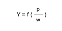
The production equation (y) is positively correlated with price levels (P) and inversely related to wages (w). Higher prices (P) lead to greater output (y), whereas higher wages (w) reduce output (y).