Producer Equilibrium

Producer equilibrium refers to the optimal combination of productive factors that a firm uses while adhering to its cost constraints. This combination allows the producer to maximize output given the available resources. Producer equilibrium represents an optimal production point and coincides with the optimal allocation of factors. Graphically, it is identified as the tangency point between the outermost isoquant curve and the producer’s isocost line.

The isocost line represents the combinations of production factors that the producer can afford within their spending capacity (C). Each point on the isocost line corresponds to a specific combination of inputs (K, L) at a constant expenditure level (C). Any combination outside the isocost line is unattainable due to insufficient financial resources. Conversely, isoquant curves depict the different combinations of inputs that yield the same level of output. Every point on an isoquant corresponds to the same production quantity (Y). The farther an isoquant is from the origin, the greater the associated level of production. At point A, the producer reaches the highest possible isoquant, maximizing output (Y₁) while fully utilizing available resources (C). At equilibrium (point A), the slope of the isocost line (marginal rate of transformation) equals the slope of the isoquant curve (marginal rate of technical substitution).

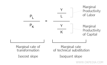
At the optimal equilibrium point, the relative prices of production factors equal the inverse ratio of their marginal productivities. If this condition were not met, the producer would adjust the input mix to maximize output while keeping costs constant (C). This economic principle becomes clearer through a few algebraic transformations.

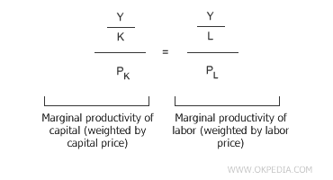
At equilibrium, the price-weighted marginal productivity of each factor must be equal (equality of marginal productivities).

MPA_K = MPA_L

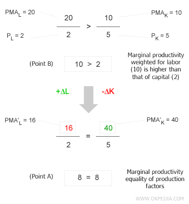
For example, if the marginal productivity of labor exceeds that of capital (MPA_L > MPA_K), the producer would benefit from increasing labor input (+ΔL) while reducing capital input (-ΔK). This adjustment would lead to a higher output level (Y) without increasing total expenditure (C). Graphically, this situation is illustrated at point B in the Cartesian diagram.

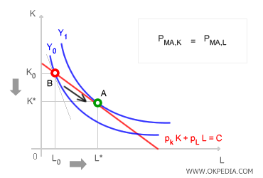
Initially, the producer is at point B, spending C to acquire a combination of inputs (L₀, K₀) and producing Y₀ units of output. However, this allocation is inefficient. At point B, the marginal productivity of labor is higher than that of capital. To optimize production, the producer increases labor input while reducing capital input. As labor input (+ΔL) rises at the expense of capital (-ΔK), the marginal productivity of labor (MPA_L) gradually declines, while that of capital (MPA_K) increases. Since these changes occur along the isocost line, total expenditure (C) remains unchanged. Over time, equilibrium shifts from point B toward point A. This process continues until the marginal productivities of both inputs, weighted by price, are equal (MPA_L = MPA_K). By the end of this adjustment, the producer achieves a higher output level (Y₁ > Y₀) while keeping costs constant (C). The new equilibrium point is A. The mathematical proof of this advantage is shown below:

Inefficient Allocations. At points B and C, the producer fully utilizes available resources, incurring a total cost of C (total cost). While these allocations respect the producer’s budget constraint, they remain inefficient because they lie on isoquant Y₀, which is closer to the origin than isoquant Y₁. This means that, despite spending the same amount (C) as in combination A, the producer obtains a lower output level (Y₀ < Y₁).

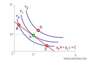
Impossible Allocations. Point D represents an economically unfeasible allocation of production factors. Every point on isoquant Y₂ lies beyond the isocost line, meaning the producer lacks the financial resources (C) to afford such combinations. Consequently, this allocation is unattainable.