Budget Constraint

The budget constraint defines the range of options available to a consumer, limited by their income or the amount of money they have. It assumes the individual has a certain income or sum of money to spend on goods and services. Given n consumption goods x and an income R, the consumer's budget constraint can be expressed as:

p₁x₁ + p₂x₂ + ... + p_nx_n ≤ R

The left side of the inequality lists the combinations of goods (or services) purchased, where x_n is the quantity of the n-th good (e.g., 5 kg of bread) and P_n is the unit price of that good (1 euro per kilogram). The right side shows the consumer's available income (R). In essence, the consumer can choose various combinations of goods as long as their total expenditure does not exceed their income (R). The prices of goods are set by the market (market prices) and are therefore known and independent of the individual consumer's choices. The income R is also a given. The only unknowns in the inequality are the variables x, representing the quantities of the n goods to be purchased. To sum up, given an income R, the consumer must choose a combination of goods—denoted as a vector (x1, x2, ... xn)—such that their total spending is less than or equal to their income.

Graphical Representation of the Budget Constraint. The budget constraint can be visually represented on a Cartesian plane. To do this, we introduce a few assumptions:

• Two-Good Budget Constraint. The consumer can choose between just two goods, x₁ and x₂ (e.g., bread and wine).
• Constant Prices and Income. Both income and prices are fixed. They are treated as external variables to focus the analysis on the consumer’s decision-making regarding the quantities of goods to purchase.

With these assumptions in place, we can plot the budget constraint on the Cartesian plane. The x-axis represents the quantities of good x₁, while the y-axis represents those of good x₂. For simplicity, we'll refer to good x₁ as good 1 and good x₂ as good 2 throughout this explanation.

Finding the Endpoints of the Budget Line. Suppose the income R is spent entirely on good 1 (bread). By allocating all income to good 1 (and none to good 2), the consumer obtains R/P1 units of good 1. This choice defines point A's coordinates on the diagram. Alternatively, if the entire income is allocated to good 2 (and none to good 1), the consumer gets R/P2 units of good 2. This choice determines point B on the Cartesian plane.

The Budget Line. To represent the budget constraint for intermediate cases, simply draw a line connecting point A to point B. This line is known as the "budget line" or "budget constraint line."

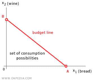
The budget line shows all the combinations in which the consumer spends their entire income on goods 1 and 2. The area below the budget line is known as the set of consumption possibilities. The line itself is called the consumption possibilities frontier, as it represents combinations (or consumption bundles) that require spending the entire income R. The area above the budget line contains choices that are out of reach for the consumer, as they exceed their income.

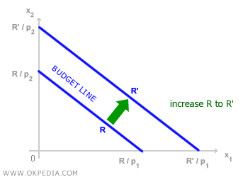
• Income Changes. An increase or decrease in income R shifts the budget line rightward or leftward, parallel to its original position. This parallel shift occurs because the ratio of the prices of goods remains unchanged.
  
• Price Changes. A change in the price ratio p₂/p₁ alters the slope of the budget constraint and its intercepts on both the x-axis and y-axis. The line rotates toward the axis of the good whose price has increased, and vice versa.
  

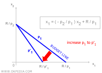
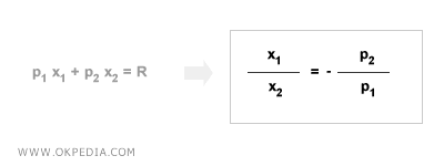
Slope of the Budget Line. The budget line slopes downward because, given a fixed income, a consumer can buy more of one good only by reducing the quantity of the other. The slope of the budget line equals the negative ratio of the goods' prices (-p₂/p₁).

Optimal Choice. The budget constraint alone does not identify the consumer's optimal choice; it merely shows the full set of possible choices. To determine the optimal choice, one must also consider the consumer's preferences and plot both the budget constraint and the indifference curves on the Cartesian plane.