Price-Consumption Curve

The price-consumption curve illustrates how consumer choices shift as the price of a good changes, displayed on a Cartesian plane. This curve helps analyze how fluctuations in a good's price influence the quantity that consumers decide to buy. For two goods, X1 and X2, priced at P1 and P2 respectively, along with a budget constraint and a set of indifference curves representing consumer preferences, consumption choices can be mapped effectively.

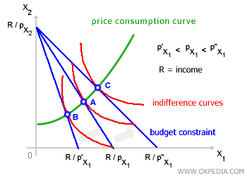
When the price P_X1 of good X₁ varies while the price P_X2 of the other good remains fixed, the budget constraint changes, shifting the boundary of affordable baskets for the consumer. For instance, an increase in P_X1 tightens this boundary (case B), while a decrease expands it (case C), moving the consumer’s choice to a more favorable, outward indifference curve. Unlike changes in income, a price change for a single good also affects the relative price between the two goods, altering the slope of the budget line. With each adjustment in relative prices, a new optimal choice point is identified, such as points A, B, and C. Connecting these optimal consumption points at various price levels of good X₁ allows us to trace the price-consumption curve on the graph.

Relative Prices. Changes in P_X1 impact not only the demand for good X₁ but also for good X₂, even if P_X2 remains constant. This happens because demand is driven by the relative price of goods, rather than just individual prices. Each shift in P_X1 thus changes the relative price P_X2 / P_X1, resulting in a new optimal combination of goods X₁ and X₂ in the consumer’s choice basket.

Intercepts. Adjustments in P_X1 change the budget line's intercept on the X₁ axis. These intercepts are determined by the ratio of the consumer’s income R to the price of the good. Each intercept reflects the maximum amount of the good that the consumer can afford given their income R and the price P. For example, an increase in the price of X₁ from P_X1 to P'_X1 reduces the maximum amount of X₁ that can be purchased with income R. Conversely, lowering the price from P_X1 to P''_X2 increases the maximum amount of X₁ purchasable with income R. Because the price P_X2 of good X₂ is assumed constant here, the intercept on the X₂ axis remains unaffected by changes in P_X1, as the quantity of X₂ that can be purchased depends solely on income R and price P_X2, as shown by the ratio R / P_X2.

Individual Demand. From this graphical representation, you can construct the consumer’s demand curve for each of the two goods. This is done by plotting the quantity demanded of the good at each optimal choice alongside its price on a Cartesian diagram.